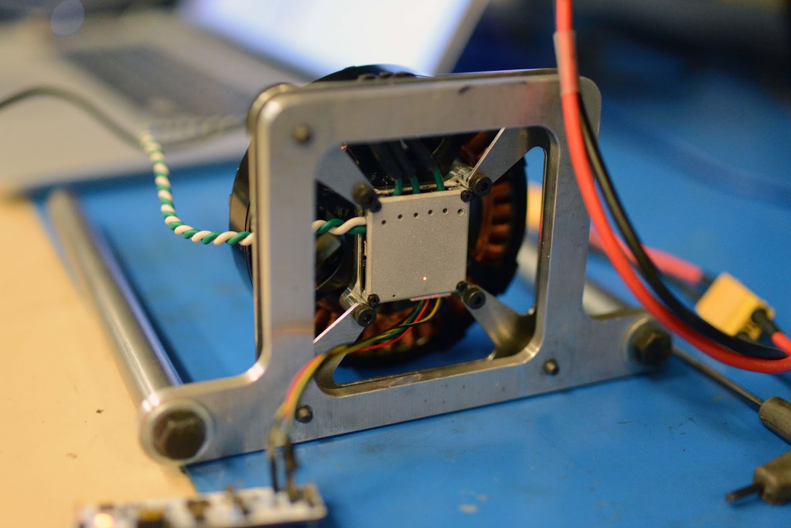
Over a year ago I started porting my motor control firmware away from mbed. I've been working on it in spurts every few months and and ended up re-doing a lot of things from scratch, so it took much longer than I originally planned. Find it here:
The core motor control math hasn't changed (foc.c is nearly identical to the old version). Lots of features have been improved though:
Encoder calibration/linearization is now current-mode, not voltage mode, and the calibration current can be configured from the serial terminal interface
Lots more parameters are configurable from the serial interface
Hardware setup is done with the Cube auto-generated setup code. Linking between the hardware and motor control code is all done in hw_config.h so it should be pretty easy to port to different micros (someday I'll switch to using G4's instead of F446's....)
It's certainly not completely polished, but I think everything's working - I've been using this firmware for the espresso machine pump. I don't have any Mini Cheetah hardware other than the motor drives any more, so I haven't been able to confirm backwards-compatibility. Let me know if you try it and have problems.
I've been working on a large robot-size motor drive, with a design target of 75V, >70A (peak phase) continuous with heatsinking, and >150A peak. In order to make the drive as compact as possible, it's split into three separate boards stacked on top of each other. The bottom layer is the power layer with MOSFETs, ceramic DC link capacitors, and current shunts. To minimize the thermal resistance between all the heat generating components to the world, the power layer is built on a 2-layer aluminum substrate board. Above the power board is the logic board with microcontroller and gate-drive, built on a normal 4-layer 1 oz board. On the very top is a breakout board with connectors for DC power input, the 3 phases, and communication/encoder
To get a better feel for how well the aluminum power board will work, I built a simple half-bridge using the same FETs as I plan on using for the final motor drive.
Here's the first test-board, affectionately named The Half Bridge of Science. It's just 2 parallel TPW3R70APL FETs per side, some 250V .47 uF ceramic caps, and a couple TLP152 gate-drive optocouplers to drive the gates.
Here's my dummy load for the half-bridge: 4 big "Pickle" resistors in a 2S2P arrangement for 1 ohm and lots of watts, with the boost converter inductor from a Ford Fusion hybrid in series.
Here it is with 55 DC amps (equivalent to 77 peak sinusoidal amps) going out of it at 50V on the input at a 50% duty cycle, basically perfectly maxing out the MITERS Lambda 50V 30A supplies.
Here are side-by-side shots of the board with a thermal camera at 55A switching at 10 kHz on the left, and 20 kHz on the right. Here's it's poorly clamped to a heatsink with no thermal paste. At 10 kHz, the FETs (Sp2) ran at 57 C, and the ceramic capacitors (Sp1) at 55. At 20 kHz, the FETs were at 65 C and the hottest of the ceramics at 75 C. Looks like I need more DC link ceramics to handle the ripple current.
There were a few mistakes with this board, so I expect thermal performance to only get better from here - I accidentally used the 1 W/m-K insulator instead of the 2 W/m-K insulator that's also available, and I misinterpreted the minimum via size, so the thermal vias were huge and sparse. This seemed pretty promising, so I designed 3-phase version
Here's the populated 3-phase power board. For testing, I got a normal FR4 board to confirm that everything works. The copper power links between the boards were custom-machined, since I couldn't find any COTS pins that were as compact.
Here's the logic board, minus gate driver. To start out, I'm trying the DRV8353S gate drive IC. It's very similar to the DRV8323 I used on my smaller motor drives. I went for the version without a built-in buck converter and use an external 15V and 5V buck to power everything. Since the DRV8323 was good for driving 2 FETs very similar to these at 40 kHz, it should be able to drive twice as many FETs at 20 kHz.
The top of the stack has Wurth terminals to get power in and out, and some JST-SH's for logic. I plan on replacing the logic connectors with something more robust like the Harwin Datamate L-Tek's I used on the Mini Cheetah, once everything is up and running.
The assembled stack:
Next time it will be a little bit thinner - I ordered the wrong male header for the board-to-board connectors, so the boards sit a little further apart than I originally intended.
Next to a coke can for a sense of scale. The footprint of the drive is 45x45mm.
Hooked into a giant T-motor U15 I'm using for testing:
That's all for now. There were two swapped pins on the logic board I had to fix with air-wires, but other than that everything seems to work. Unfortunately I made some dumb testing mistakes and blew up the controller before I could push it too hard, and the stacked construction is almost impossible to disassemble. But now that I know the board layout works I'm going to send out for the aluminum power boards. Stay tuned.
I just finished building a bunch of Mini Cheetahs which the lab is loaning out to other research groups. Since we're giving these to people who for the most part aren't hardware oriented, these robots need to be even more robust than the original one.
One piece of that is preventing the motors from burning out. During normal operation with a good locomotion controller, the motors barely even get above ambient (even going 3.7 m/s, the motors weren't warm to the touch afterwards). However, it's really easy to write a controller that rapidly heats up the motors without actually doing anything - railing torque commands back-and-forth due to instability, joints mechanically stuck against something, machine-learning algorithm flailing around wildly, etc. We haven't burned out any motors on the original Mini Cheetah yet, but I think our lab members all have a pretty good sense of what's good/bad for the robot, and know to shut it down quickly if something bad is happening. But when the robot is in the hands of a bunch of software and machine learning engineers..... So to protect the robots, I'm adding in winding temperature sensing and over-temperature protection, to (hopefully) make it impossible to burn out the motors.
Now, the smart way to do this would have probably been to just add a thermistor in the windings, and call it done. Obviously, I didn't do that, so here's my observer-based workaround.
Overview
The temperature estimate uses an observer to combine two sources of information: A thermal model of the motor, and a temperature "measurement" based on the resistance temperature coefficient of the copper in the windings. The resistance of the motor is estimated based on applied voltage, measured current, measured speed and known motor parameters, and compared against the resistance at a known temperature. Sounds pretty simple, right?
Of course not. If it was, it wouldn't be worth a blog post. It's not terribly complicated either, but it took a bunch of little hacks to make it actually work.
Thermal Modeling:
I'm using a 1st order thermal model with just thermal mass \(C_{th}\) and thermal resistance to ambient \(R_{th}\). With temperature rise over ambient \(\Delta T\), thermal power going in \(\dot{Q_{in}}\), and thermal power going out \(\dot{Q_{out}}R_{th} = \Delta T\), the dynamics are
$$
\Delta \dot{T} = \frac{\dot{Q}_{in} - \dot{Q}_{out}}{C_{th}}
$$
To get \(\dot{Q}_{in}\), I just use \(i^{2} R\), but accounting for the variation from nominal resistance\(R_{0}\) due to \(\Delta T\), i.e. it's temperature coefficient of resistance \(\alpha\) (.00393 for copper):
$$
\dot{Q}_{in} = (1 + \alpha\Delta T)R_{0}i^{2}
$$
In (slightly simplified) code, the model part of the observer is updated as follows, by Euler-integrating the thermal model.
An important implementation detail, in the actual firmware I'm doing the last line of math as doubles, rather than floats like everything else. My sample period DT is very small (since my loops run at 20-40 kHz depending on the motor I'm driving), and \( \frac{\dot{Q_{in}} - \dot{Q_{out}}}{C_{th}}\) is also pretty small since the thermal dynamics are very slow. As a result, the change in temperature over one loop-cycle gets rounded down to zero when you use floats. Since STM32F4's are crap-tastic at double math, this single line takes a substantial fraction of my 25 microsecond loop period when I'm running at 40 kHz. I'm sure there's a way to do this avoiding doubles, but I have just enough computational headroom that I don't care.
Measuring Temperature and Resistance
Assuming we can measure the resistance of the motor perfectly and we know nominal resistance \(R_{0}\) at some temperature \(T_{0}\), and the temperature coefficient \(\alpha\) , we can calculate temperature:
$$
T = T_{0} + \left(\frac{R}{R_{0}} -1 \right)\frac{1}{\alpha}
$$
To measure \(R\), use one of the synchronous motor voltage equations. I use the Q-axis one, because for my surface PM robot motors there's usually not much current on the D axis.
We'll assume \( \frac{di_{q}}{dt} \) is zero, since the temperature observer is going to be very low-bandwidth compared to the current control dynamics. Conveniently if you use the Q-axis voltage equation rather than the D-axis one, the \( \omega L_{d}i_{d} \) term is usually zero, since \(i_{d} \) is only non-zero at high-speeds during field weakening, and in that region you can't get enough q-current into the motor to burn it out anyways.
Since we know \(V_{q}\), \(i_{q}\), \(i_{d}\), \(\omega\), \(l_{d}\), and \(\lambda\), we can just solve the voltage equation for \(R\). In reality I had to add a trick to get this to work, but I'll get into that later.
Implementing the Observer
The basic steps in the observer are:
Integrate forward the dynamics of the quantity you are estimating
Take a sensor reading and calculate the error between the estimate and the sensor reading
Use a proportional controller to drive the estimate towards the sensor reading
In code the whole observer looks like this:
// Integrate the thermal model //delta_t=observer.temperature-T_AMBIENT;observer.qd_in=R_NOMINAL**(1.0f+.00393f*delta_t)*controller.i*controller.i;observer.qd_out=delta_t*R_TH;observer.temperature+=DT*(observer.qd_in-observer.qd_out)/C_TH;// Estimate Resistance //observer.resistance=(controller.v_q- controller.omega*(L_D*controller.i_d+WB))/(controller.i_q);// Estimate Temperature from temp-co //observer.t_measured=((T_AMBIENT+((observer.resistance/R_NOMINAL)-1.0f)*254.5f));// Update Observer with measured temperature //e=(float)observer.temperature-observer.temp_measured;observer.temperature-=.0001f*e;
Naively implemented, the above didn't really work - the resistance measurements are terrible , so either you have a very low observer gain and basically run open-loop with just the thermal model, or the temperature estimate varies wildly depending on the speed and torque the motor is operating at. It took a couple more additions to get it to work reliably.
Voltage Linearization
The first problem I notice was that the measured resistance changed dramatically as the current varied. At low currents, the estimated resistance was much higher. This problem was caused by nonlinearity in the voltage output of the motor drive due to deadtime. I tried a few methods for compensating the dead time, but I got the best result by scaling my d and q axis voltages based on modulation depth. I measured the nonlinearity by logging measured current vs commanded modulation depth over a range of currents, putting all the current on the d-axis so the rotor didn't move.
I generated a lookup table to scale the commanded voltages so that current vs commanded voltage is linear. Around zero commanded voltage, I actually only get about .5 output volts per commanded volt, pre-linearization:
State-dependent Gain Scaling
i.e. lazy person's Kalman filter substitute.
Even with the voltage linearization, there are some operating conditions which make it hard to measure the resistance accurately.
At very low currents the measurements are bad. You have a small voltage divided by a small current, so the result is super sensitive to noise or bias in either.
At high speeds the measurements are also bad since the flux linkage term in the voltage equation dominates. Slight error in the flux linkage constant causes errors, and also non-sinusoidal flux linkage and inductances mean there's lots of ripple in the d and q voltages and currents at high speed.
The least sketchy way to incorporate these effects might be to figure out how the covariance of the temperature "measurement" depends on the operating state, and use a Kalman filter to optimize the observer gain based on the changing covariance.
My sketchy alternative was to hand-tune a "trust" function which behaves similarly to inverse covariance, to make the gain really small in states where I don't trust the temperature measurement. Basically, if the current is below some threshold, make the gain really small, and/or if the speed is above some threshold, make the gain really small. Around each threshold I have a linear ramp, to smooth things out a bit. In code, my "trust" function works like this:
// Calculate "trust" based on state //observer.trust=(1.0f-.004f*fminf(abs(controller.dtheta_elec),250.0f))*(.01f*(fminf(controller.current^2,100.0f)));// Scale observer gain by "trust" //// .0001 is the default observer gain //observer.temperature-=observer.trust*.0001f*e;
When the resistance estimates are the best (current greater than 10 amps, speed near zero), "trust" is equal to 1, so the observer gain doesn't change, and the observer gain goes to zero (i.e. open-loop) at really bad measurement points. I'm sure this would horrify every controls professor I've had, but it works pretty well:
Here's a video of testing with one of the mini cheetah motors, with a thermocouple glued into the windings. I'm railing the current command between -40A and 40A at 5 hz, so the motor only spends a very brief period of time at low speed, and most of its time at high speed with low current. In this test I initialize the motor temperature at 25 degrees, even though the motor is still at 60 degrees from a previous experiment. The observer takes about 16 seconds to converge to the actual temperature, but from there on it tracks to within ~5 degrees. Once the temperature hits 120 degrees, the current limit is throttled back to 14 amps in order to keep the temperature below 120 C:
I was playing with my thermal test motor, and noticed that at high speeds, some pretty significant harmonics showed up in the phase currents. Here's an example with an obvious 5th harmonic - I'm commanding 20A, peak, and the harmonics add a couple amps of ripple on top of that:
This ripple shows up because there's a 5th harmonic in the motor's flux linkage (and therefore back-emf). From the perspective of the field-oriented control, these harmonics at the phases show up as AC disturbances on the D/Q voltages. The two current loops will try to squash these disturbances, but it's ability to do so depends on the current loop bandwidth and the magnitude of the disturbances. Since both the magnitude and frequency go up with motor speed, even really high-bandwidth current loops have trouble keeping up. For example, in the scope shot at the top, the current loop had around 2 kHz closed-loop bandwidth. The motor's electrical frequency was 300 Hz, so the harmonic (in D/Q) was at 1.8 kHz, so the controller couldn't quite reject it.
So how exactly do harmonics in the flux linkage at each phase show up when transformed into D and Q? In the sinusoidal flux linkage case with no position-varying inductance, the motor's dynamics in the D/Q frame is exactly the classic voltage equations:
Where \(L\) is the synchronous inductance, \(R\) is the synchronous resistance, \(\omega\) is the (electrical) angular velocity, and \(\lambda\) is the peak flux linkage of one phase.
In the equations above, the flux linkage of a single phase \(\lambda_{p}\) is assumed to be of the form \(\lambda_{p} = \lambda \cos(\theta)\), where \(\theta\) is the rotor angle. Other phases will have an offset of \(\pm \frac{2\pi}{3}\).
If the flux linkage has a fifth-harmonic in it, for a single phase it looks like \(\lambda \cos(\theta) + \lambda_{2}\cos(5 \theta) \). With the fifth harmonic in flux linkage, the voltage equations in D and Q become:
(I have no interest in doing tedious trig and algebra by hand, so I wrote a Mathematica script to do the transforms analytically for me.)
That's interesting - a fifth harmonic at the phases shows up as a 6th harmonic through the transforms. It turns out, a 7th harmonic at the phases also shows up as a 6th harmonic through the transforms - just with both positive sine and cosine components, rather than positive sine negative cosine. 11 and 13 show up as 12, and so on. Also (although this may be more intuitively obvious), odd multiples of 3 disappear through the transforms.
Just to confirm, here's the output when plugging a fifth harmonic into my motor simulator, using the the other motor parameters from the U12 and same controller gains as the hardware.
Phase currents:
D and Q axis currents, as well as rotor angle. You can count the 6 periods in the AC component of the current per electrical cycle.
So what if you want to control out those harmonics? Or add in harmonics of your own, for some reason? If you know how the voltages of the harmonics appear on the D and Q axes, theoretically you could feed-forward them out, but there's a more interesting way to closed-loop deal with them, without knowing the specific amplitude of phasing of the harmonic, just it's frequency.
Introducing Adaptive Feedforward Cancellation. This is a weird technique which was briefly introduced at the very end of 2.14, which has the seemingly magical property of giving your controller infinite gain at a specific frequency - i.e. it will perfectly track a signal at that frequency, or perfectly reject a disturbance at that frequency. AFC is probably most well-known for its use in things like hard-disk read heads, which have to follow very fine tracks of data on the hard drive platters. Since the platters have some runout as they spin, the read-head has to track in the presence of periodic disturbances. Interestingly, AFC is a lot like field oriented control: FOC gives your controller infinite gain at the fundamental electrical frequency of your motor, letting you track sinusoidal currents of much higher frequency than the bandwidth of your current controllers.
Here's a block diagram of how AFC works, taken from the paper "Adaptive feedforward cancellation viewed from an oscillator amplitude control perspective". \(r(t)\) is the reference (current, in my case), and \(d(t)\) is a disturbance (back-emf harmonics, in my case), and \(y(t)\) is the control effort (D or Q voltage in my case).
And here's how the AFC(s) are integrated into the control loop. The red box is your normal feedback controller (in my case the PI current controllers for D and Q current).
The AFC works kind of like a pair of integrators on the sine and cosine components of the periodic part of the error. If there's zero error \(e(t)\), the AFC outputs the sum of \(\cos(\omega t)\cdot (\text{cos integral})\) and \(\sin(\omega t)\cdot (\text{sin integral})\), which is some sinusoidal thing. If there is some error, the portion of it at the same frequency as \(\omega\) doesn't average to zero when multiplied by the \(\cos(\omega t)\) or \(\sin(\omega t)\)'s before the integrators. The integrators then integrate up to whatever value drives the \(\omega\) frequency component of the error to zero.
The slight modification to get this to work for motor currents is changing the \(\omega t\) to be \(\theta\), the electrical angle of the motor. The periodic disturbances are not a fixed frequency in time, they are a fixed frequency in state.
This basically just works. Implementing a 6th harmonic AFC on both the D and Q current loops completely eliminates the 5th harmonic in phase currents. Here's the simulation result:
Phase currents:
D/Q currents:
And here's what the integrators in the AFC do:
There's one simple addition to the controller which makes it behave a little better. The magnitude of the harmonic voltage is proportional to how fast the motor is spinning - so if the motor is accelerating, the magnitude is increasing, and the AFC integrators are constantly playing catch-up. This means that at a constant acceleration, there will be a constant error in the AFC:
The AFC still does a pretty good job even at high acceleration, but how well it does depends on how large the AFC gain is. Below you can see the integrators ramping up with speed:
The simple fix for this is to divide the error by angular velocity before integrating, and then multiply by angular velocity at the end of the AFC calculations. This way, the AFC integrators integrate up to the harmonic in the flux linkage, which is constant, rather than the back-emf, which is proportional to speed. Honestly, this change doesn't make a huge difference, because the time constant of the integrator can be quite fast compared to how fast the motor can accelerate, but it's kind of cool none the less:
Now the integrators just converge to constants, even as the motor accelerates:
Pseudo-code implementation:
 1
 2
 3
 4
 5
 6
 7
 8
 9
10
11
12
13
14
15
h=6.0f;// Harmonic numberk_afc=100;// AFC Gain - larger gain converges fasters=sin(h*theta);c=cos(h*theta);i_error=i_ref-i;if(abs(thetadot)>1)//avoid dividing by zero{afc_cos_int+=dt*i_error*k_afc*c/thetadot;afc_sin_int+=dt*i_error*k_afc*s/thetadot;}afc_out=thetadot*(s*afc_sin_int+c*afc_cos_int);i_error=i_ref-i+afc_out;//Now use this error in the PI current loop.
And here it is after implementing on the hardware:
The AFC behaves a little strangely when the voltage saturates (causing higher harmonics to show up), and I haven't put any effort into fixing that, but for most operating points it works quite well.
Here's an FFT of the phase current at the beginning of the post. There are significant components at 5, 7 and 11 times the electrical frequency:
And here's the FFT after adding an AFC at 6 times the electrical frequency:
In addition to canceling out harmonics, you can use this technique to add in harmonics of your own, or track periodic current references.
For example, a typical way to cancel out cogging torque is to add in an AC component to your Q-axis current reference which tries to cancel out the cogging torque. The controller's ability to track this reference depends on how fast the motor is spinning, and its bandwidth. But if you add in an AFC at the cogging frequencies, the AFC just takes care of tracking the cogging current.
Or if you want to add certain harmonics at the phases, you can do so by taking the dq0 transform of the harmonics you want, then adding those to your D/Q current references with an AFC to track them. Say, for example, you wanted your phase currents to be more trapezoidal, you could take the transform of the trapezoidal waveform, use that as your D/Q current references, and add AFCs at the first few Fourier coefficients in order to track the reference at high speed.
I made a cover for the small motor controller, which serves as both a top-side heatsink for the MOSFETS and gate driver, and (more importantly) as a clamping mechanism to keep the PCB flat and evenly pressed against the heatspreader beneath it.
In the picture below, the heatspreader is on the left, and cover on the right: The bar across the bottom sits on top of the FETS, the square in the middle sits above the DRV chip. I left a 0.1mm gap between the FET-bar and the top of the FET package, which gets filled by some .5mm thermal pad. This allows for some variation in the height of the transistors once they're soldered down, and the compression of the thermal pad means there's a fair amount of pressure pushing down on the top of each transistor.
Motor Controller Sandwich:
The two little holes let through light from the two indicator LEDs on the board.
I made a Special Motor Controller Cover of Science to help out with thermal camera-ing. It has a 1.5mm hole drilled above the center of each transistor, so that I can see through the cover with the camera. I stuck it on the same controller and motor I used for the last round of testing. I was able to use a needle to cut away the circle of thermal pad at the bottom of each hole, so you can see straight through to the tops of the FET packages.
Here's an example image You can see the transistors clearly through the holes. The bright spot on the cover where point Sp2 is is where I applied some matte black paint to get the emissivity of the aluminum cover closer to 1.
The cover was extremely effective. Here's a 30A test. By the time the motor windings reached 70 C, the FETs were all under 48 C, and there was only a 1.6 C difference between the hottest and coldest transistors. For reference, in my last tests without the cover, by the time the motor reached 70 C at 30 amps, the FETs were between 67 and 72 C.
Going a little harder, here's after running 33 A until the motor windings reached a rather uncomfortable 80 C. There's a 5 degree drop between the top of the transistor and the surface of the cover.
With the various layout errors on the last set of boards fixed, the controller seems to work as expected, so I've been doing some thermal testing.
I strapped the controller to a much bigger motor: Even with the old version of the controller, the small motors I've been using would catch on fire before the controller does.
Here it is attached to a T-motor U12:
The test setup, with the motor and controller in view of Bayley's thermal camera
For the first tests, I put the test current on the d-axis, and 2A on the q-axis just to get the motor spinning.
Originally, I had a 0.5mm layer of thermal pad between the board and an aluminum heatspreader and aluminum motor mount beneath.
At 15 amps, basically nothing happened. I made the passives for the buck converter and the 3.3V linear regulator much smaller on this board, so it was good to see that they're doing fine.
At 20 A you could start to see the FETS getting warm.
And here's 30A. I only let this one run for around 30 seconds. The FETs in the middle of the board are noticeably hotter than those by the edges, which I partially blame on poor contact with the thermal pad. Since the screws are at the edges of the board, the board flexes when they are tightened, and all the clamping pressure is at the corners. Also interesting, it looks like the trace from the source of the FET in the bottom right corner is getting pretty warm. The hole for the mounting screw makes the phase polygon pretty narrow there. I should be able to fix that by adding a row of vias from the source legs to the internal phase layer (which I should have added before). These boards only have 1 oz copper on top and bottom, and 1.5 oz internal layers.
And the plots. With this setup, I wouldn't be comfortable running the controller at 30A continuous.
I switched out the thermal pad for a layer of kapton tape for electrical insulation, and some thermal paste. Contact in the middle was still not great, but overall it was a lot better than the thermal pad.
Performance was greatly improved, but there's still a ~7 degree C difference between the hottest and coldest FETs. Furthermore, in the middle of the board, the low-side FETs are several degrees hotter than the high-side FETs - traces Sp3 and Sp2 respectively on the plot below:
It looks like with this setup, the controller can handle around 30A continuously. I'm pretty satisfied with that, but I think the performance would be substantially improved by adding an aluminum cover over the motor controller which firmly pressed against the row of FETS, to get good contact on the bottom of the board. The cover would also serve as a top-side heatsink, which is surprisingly effective with this FET package, as there's only ~0.3mm of plastic above the copper clip on top of the die (I sanded one down to measure).
I've been using these 3.3 mOhm fets, which I like because they're cheap and have only 50 nC gate charge, so they don't stress the DRV chip switching at 40 kHz. I swapped out the FETs for the 1.4 mOhm flavor, since I had a bunch of them lying around. These have ~half the resistance, but about twice the gate charge, so twice the switching loss. It works out slighly favorably in this case (for currents above around 20A) - I expect around 10% less dissipation per-fet at 30A.
Here's 30A on the 1.4 mOhm FETs. Check out how much hotter the DRV chip gets, doing twice the gate drive work. ~10 C hotter than before. There are actually lots of better transistors available now, even for similar price, so I can get power dissipation down around 15-20% further.
To make the tests a bit more stressful, I put the motor on the dyno so I could actually get some power into and out of it. I made a new motor mounting plate which doesn't cover up the controller:
This time, I put all 30A on the Q-axis, and ramped up the speed until the achievable current just started to drop off (which is the maximum power point for this motor). At 22V on the bus, I was able to put 500 watts in and get 400 back out. I let everything cook for a while to get up to temperature. The only noticeable difference was that the DC link wires were roasting. The 16 AWG is not really meant for 23A DC + ripple current in continuous duty. Going into this test, I was a little worried about how the ceramic DC link capacitors would handle the current ripple, since there's only 60 uF on the board, but they didn't get any hotter.
To see where all the temperature drop was coming from, I got a side-view of the heatspreader and motor mount assembly. Point Sp3 is on the side of the motor mount, point Sp2 is on the side of the heatspreader, Sp1 is the hot FET, and Sp4 and 5 are the cooler FETs. This is after running for several minutes continuously at 30 A
The heatspreader, motor mount, and the back of the motor were all within a couple degrees of each other, with all the temperature drop happening between the FETs and the heatspreader.
With an estimated power dissipation of 1 watt per FET at 30A, this gives a thermal resistance of 12 C/watt between the transistor and the heatspreader for the cooler FET, and 17 for the hot one.
Here's a sketched cross section of the 3 different FET layouts on the board, and why I think the low-side FETs with shunts get so much warmer than the others (in addition to the poor clamping at the middle of the board).
First, the high-side FETs, which are the coolest. Labeled stack-up on the left, main heat conduction path on the right. The vias beneath the drain tab go straight into the big V+ plane on the bottom, which is copper, so super thermally conductive in the plane. This effectively increases the area which conducts through to the heatspreader.
The low-side FET without the shunt, which was much cooler than the other two, looks like this: It has a bunch of vias from the source pins straight into the ground plane, in addition to the vias beneath the drain tab. The source pins are part of a monolithic copper sheet ("clip") which sandwiches the top of the die, so they can very effectively sink heat away from the die.
And finally the low-side FETs with shunts, which get kind of screwed, with no big plane beneath them, and a shunt attached to the source pins:
One way to help out those FETs might be to add some extra heat-sinking planes on the bottom of the board, like this:
But more importantly than trying to tweak the board layout to slightly improve the thermal performance, where is all the thermal resistance coming from in the first place?
According to the FET datasheet, the package to base thermal resistance is around 1.2 C/W.
I got in touch with PCBWay, and their via plating thickness is 18-22 microns, independent of the copper plating thickness. According to the Via calculator, the resistance of the patch of drain vias should be 4.6 C/W.
There's also a layer of 1 mil Kapton tape, electrically insulating the heatspreader. But the total thickness of the tape, including the adhesive, is 3 mil, or 75 microns. The 5x5m mpatch under each FET has the thermal resistance of around 6.5 C/W.
Ignoring the thermal paste, that's up to 12.3 C/W, which is right in line with the results from the thermal camera.
So the Kapton is the biggest culprit here. I'd like to try using a hard-anodized aluminum heatspreader with no additional electrical insulation. The hard anodized coating is only 0.5-1 W/m*k, but it can be very thin.
The next biggest resistance source is the vias. The PCBWay via plating thickness corresponds to a little over 1/2 oz, but I could probably do better with some other PCB manufacturer.
Also worth noting, all these tests were with no airflow over the controller. Pointing a good blower at the back dropped the temperatures by around 20C.
Next hardware steps: wait for AMS position sensors and DRV8323RS chips to come back in stock, design a FET-clamping cover, and experiment a bit more with heatsinking.