

November 7, 2019
October 31, 2019
Motor Temperature Estimation Without a Sensor
I just finished building a bunch of Mini Cheetahs which the lab is loaning out to other research groups. Since we're giving these to people who for the most part aren't hardware oriented, these robots need to be even more robust than the original one.
One piece of that is preventing the motors from burning out. During normal operation with a good locomotion controller, the motors barely even get above ambient (even going 3.7 m/s, the motors weren't warm to the touch afterwards). However, it's really easy to write a controller that rapidly heats up the motors without actually doing anything - railing torque commands back-and-forth due to instability, joints mechanically stuck against something, machine-learning algorithm flailing around wildly, etc. We haven't burned out any motors on the original Mini Cheetah yet, but I think our lab members all have a pretty good sense of what's good/bad for the robot, and know to shut it down quickly if something bad is happening. But when the robot is in the hands of a bunch of software and machine learning engineers..... So to protect the robots, I'm adding in winding temperature sensing and over-temperature protection, to (hopefully) make it impossible to burn out the motors.
Now, the smart way to do this would have probably been to just add a thermistor in the windings, and call it done. Obviously, I didn't do that, so here's my observer-based workaround.
Overview
The temperature estimate uses an observer to combine two sources of information: A thermal model of the motor, and a temperature "measurement" based on the resistance temperature coefficient of the copper in the windings. The resistance of the motor is estimated based on applied voltage, measured current, measured speed and known motor parameters, and compared against the resistance at a known temperature. Sounds pretty simple, right?
Of course not. If it was, it wouldn't be worth a blog post. It's not terribly complicated either, but it took a bunch of little hacks to make it actually work.
Thermal Modeling:
I'm using a 1st order thermal model with just thermal mass \(C_{th}\) and thermal resistance to ambient \(R_{th}\). With temperature rise over ambient \(\Delta T\), thermal power going in \(\dot{Q_{in}}\), and thermal power going out \(\dot{Q_{out}}R_{th} = \Delta T\), the dynamics are
$$
\Delta \dot{T} = \frac{\dot{Q}_{in} - \dot{Q}_{out}}{C_{th}}
$$
To get \(\dot{Q}_{in}\), I just use \(i^{2} R\), but accounting for the variation from nominal resistance\(R_{0}\) due to \(\Delta T\), i.e. it's temperature coefficient of resistance \(\alpha\) (.00393 for copper):
$$
\dot{Q}_{in} = (1 + \alpha\Delta T)R_{0}i^{2}
$$
In (slightly simplified) code, the model part of the observer is updated as follows, by Euler-integrating the thermal model.
An important implementation detail, in the actual firmware I'm doing the last line of math as doubles, rather than floats like everything else. My sample period DT is very small (since my loops run at 20-40 kHz depending on the motor I'm driving), and \( \frac{\dot{Q_{in}} - \dot{Q_{out}}}{C_{th}}\) is also pretty small since the thermal dynamics are very slow. As a result, the change in temperature over one loop-cycle gets rounded down to zero when you use floats. Since STM32F4's are crap-tastic at double math, this single line takes a substantial fraction of my 25 microsecond loop period when I'm running at 40 kHz. I'm sure there's a way to do this avoiding doubles, but I have just enough computational headroom that I don't care.
Measuring Temperature and Resistance
Assuming we can measure the resistance of the motor perfectly and we know nominal resistance \(R_{0}\) at some temperature \(T_{0}\), and the temperature coefficient \(\alpha\) , we can calculate temperature:
$$
T = T_{0} + \left(\frac{R}{R_{0}} -1 \right)\frac{1}{\alpha}
$$
To measure \(R\), use one of the synchronous motor voltage equations. I use the Q-axis one, because for my surface PM robot motors there's usually not much current on the D axis.
$$
V_{q} = Ri_{q} + L_{q}\frac{di_{q}}{dt} + \omega L_{d}i_{d} + \omega\lambda
$$
We'll assume \( \frac{di_{q}}{dt} \) is zero, since the temperature observer is going to be very low-bandwidth compared to the current control dynamics. Conveniently if you use the Q-axis voltage equation rather than the D-axis one, the \( \omega L_{d}i_{d} \) term is usually zero, since \(i_{d} \) is only non-zero at high-speeds during field weakening, and in that region you can't get enough q-current into the motor to burn it out anyways.
Since we know \(V_{q}\), \(i_{q}\), \(i_{d}\), \(\omega\), \(l_{d}\), and \(\lambda\), we can just solve the voltage equation for \(R\). In reality I had to add a trick to get this to work, but I'll get into that later.
Implementing the Observer
The basic steps in the observer are:
Naively implemented, the above didn't really work - the resistance measurements are terrible , so either you have a very low observer gain and basically run open-loop with just the thermal model, or the temperature estimate varies wildly depending on the speed and torque the motor is operating at. It took a couple more additions to get it to work reliably.
Voltage Linearization
The first problem I notice was that the measured resistance changed dramatically as the current varied. At low currents, the estimated resistance was much higher. This problem was caused by nonlinearity in the voltage output of the motor drive due to deadtime. I tried a few methods for compensating the dead time, but I got the best result by scaling my d and q axis voltages based on modulation depth. I measured the nonlinearity by logging measured current vs commanded modulation depth over a range of currents, putting all the current on the d-axis so the rotor didn't move.

I generated a lookup table to scale the commanded voltages so that current vs commanded voltage is linear. Around zero commanded voltage, I actually only get about .5 output volts per commanded volt, pre-linearization:

When the resistance estimates are the best (current greater than 10 amps, speed near zero), "trust" is equal to 1, so the observer gain doesn't change, and the observer gain goes to zero (i.e. open-loop) at really bad measurement points. I'm sure this would horrify every controls professor I've had, but it works pretty well:
Here's a video of testing with one of the mini cheetah motors, with a thermocouple glued into the windings. I'm railing the current command between -40A and 40A at 5 hz, so the motor only spends a very brief period of time at low speed, and most of its time at high speed with low current. In this test I initialize the motor temperature at 25 degrees, even though the motor is still at 60 degrees from a previous experiment. The observer takes about 16 seconds to converge to the actual temperature, but from there on it tracks to within ~5 degrees. Once the temperature hits 120 degrees, the current limit is throttled back to 14 amps in order to keep the temperature below 120 C:
One piece of that is preventing the motors from burning out. During normal operation with a good locomotion controller, the motors barely even get above ambient (even going 3.7 m/s, the motors weren't warm to the touch afterwards). However, it's really easy to write a controller that rapidly heats up the motors without actually doing anything - railing torque commands back-and-forth due to instability, joints mechanically stuck against something, machine-learning algorithm flailing around wildly, etc. We haven't burned out any motors on the original Mini Cheetah yet, but I think our lab members all have a pretty good sense of what's good/bad for the robot, and know to shut it down quickly if something bad is happening. But when the robot is in the hands of a bunch of software and machine learning engineers..... So to protect the robots, I'm adding in winding temperature sensing and over-temperature protection, to (hopefully) make it impossible to burn out the motors.
Now, the smart way to do this would have probably been to just add a thermistor in the windings, and call it done. Obviously, I didn't do that, so here's my observer-based workaround.
Overview
The temperature estimate uses an observer to combine two sources of information: A thermal model of the motor, and a temperature "measurement" based on the resistance temperature coefficient of the copper in the windings. The resistance of the motor is estimated based on applied voltage, measured current, measured speed and known motor parameters, and compared against the resistance at a known temperature. Sounds pretty simple, right?
Of course not. If it was, it wouldn't be worth a blog post. It's not terribly complicated either, but it took a bunch of little hacks to make it actually work.
Thermal Modeling:
I'm using a 1st order thermal model with just thermal mass \(C_{th}\) and thermal resistance to ambient \(R_{th}\). With temperature rise over ambient \(\Delta T\), thermal power going in \(\dot{Q_{in}}\), and thermal power going out \(\dot{Q_{out}}R_{th} = \Delta T\), the dynamics are
$$
\Delta \dot{T} = \frac{\dot{Q}_{in} - \dot{Q}_{out}}{C_{th}}
$$
To get \(\dot{Q}_{in}\), I just use \(i^{2} R\), but accounting for the variation from nominal resistance\(R_{0}\) due to \(\Delta T\), i.e. it's temperature coefficient of resistance \(\alpha\) (.00393 for copper):
$$
\dot{Q}_{in} = (1 + \alpha\Delta T)R_{0}i^{2}
$$
In (slightly simplified) code, the model part of the observer is updated as follows, by Euler-integrating the thermal model.
delta_t = observer.temperature - T_AMBIENT;
observer.qd_in = R_NOMINAL**(1.0f + .00393f*delta_t)*controller.i*controller.i;
observer.qd_out = delta_t*R_TH;
observer.temperature += DT*(observer.qd_in-observer.qd_out)/C_TH;
An important implementation detail, in the actual firmware I'm doing the last line of math as doubles, rather than floats like everything else. My sample period DT is very small (since my loops run at 20-40 kHz depending on the motor I'm driving), and \( \frac{\dot{Q_{in}} - \dot{Q_{out}}}{C_{th}}\) is also pretty small since the thermal dynamics are very slow. As a result, the change in temperature over one loop-cycle gets rounded down to zero when you use floats. Since STM32F4's are crap-tastic at double math, this single line takes a substantial fraction of my 25 microsecond loop period when I'm running at 40 kHz. I'm sure there's a way to do this avoiding doubles, but I have just enough computational headroom that I don't care.
Measuring Temperature and Resistance
Assuming we can measure the resistance of the motor perfectly and we know nominal resistance \(R_{0}\) at some temperature \(T_{0}\), and the temperature coefficient \(\alpha\) , we can calculate temperature:
$$
T = T_{0} + \left(\frac{R}{R_{0}} -1 \right)\frac{1}{\alpha}
$$
To measure \(R\), use one of the synchronous motor voltage equations. I use the Q-axis one, because for my surface PM robot motors there's usually not much current on the D axis.
$$
V_{q} = Ri_{q} + L_{q}\frac{di_{q}}{dt} + \omega L_{d}i_{d} + \omega\lambda
$$
We'll assume \( \frac{di_{q}}{dt} \) is zero, since the temperature observer is going to be very low-bandwidth compared to the current control dynamics. Conveniently if you use the Q-axis voltage equation rather than the D-axis one, the \( \omega L_{d}i_{d} \) term is usually zero, since \(i_{d} \) is only non-zero at high-speeds during field weakening, and in that region you can't get enough q-current into the motor to burn it out anyways.
Since we know \(V_{q}\), \(i_{q}\), \(i_{d}\), \(\omega\), \(l_{d}\), and \(\lambda\), we can just solve the voltage equation for \(R\). In reality I had to add a trick to get this to work, but I'll get into that later.
Implementing the Observer
The basic steps in the observer are:
- Integrate forward the dynamics of the quantity you are estimating
- Take a sensor reading and calculate the error between the estimate and the sensor reading
- Use a proportional controller to drive the estimate towards the sensor reading
// Integrate the thermal model //
delta_t = observer.temperature - T_AMBIENT;
observer.qd_in = R_NOMINAL**(1.0f + .00393f*delta_t)*controller.i*controller.i;
observer.qd_out = delta_t*R_TH;
observer.temperature += DT*(observer.qd_in-observer.qd_out)/C_TH;

// Estimate Resistance //
observer.resistance = (controller.v_q - controller.omega*(L_D*controller.i_d + WB))/(controller.i_q);

// Estimate Temperature from temp-co //
observer.t_measured = ((T_AMBIENT + ((observer.resistance/R_NOMINAL) - 1.0f)*254.5f));

// Update Observer with measured temperature //
e = (float)observer.temperature - observer.temp_measured;
observer.temperature -= .0001f*e;
Naively implemented, the above didn't really work - the resistance measurements are terrible , so either you have a very low observer gain and basically run open-loop with just the thermal model, or the temperature estimate varies wildly depending on the speed and torque the motor is operating at. It took a couple more additions to get it to work reliably.
Voltage Linearization
The first problem I notice was that the measured resistance changed dramatically as the current varied. At low currents, the estimated resistance was much higher. This problem was caused by nonlinearity in the voltage output of the motor drive due to deadtime. I tried a few methods for compensating the dead time, but I got the best result by scaling my d and q axis voltages based on modulation depth. I measured the nonlinearity by logging measured current vs commanded modulation depth over a range of currents, putting all the current on the d-axis so the rotor didn't move.
I generated a lookup table to scale the commanded voltages so that current vs commanded voltage is linear. Around zero commanded voltage, I actually only get about .5 output volts per commanded volt, pre-linearization:
State-dependent Gain Scaling
i.e. lazy person's Kalman filter substitute.
Even with the voltage linearization, there are some operating conditions which make it hard to measure the resistance accurately.
- At very low currents the measurements are bad. You have a small voltage divided by a small current, so the result is super sensitive to noise or bias in either.
- At high speeds the measurements are also bad since the flux linkage term in the voltage equation dominates. Slight error in the flux linkage constant causes errors, and also non-sinusoidal flux linkage and inductances mean there's lots of ripple in the d and q voltages and currents at high speed.
The least sketchy way to incorporate these effects might be to figure out how the covariance of the temperature "measurement" depends on the operating state, and use a Kalman filter to optimize the observer gain based on the changing covariance.
My sketchy alternative was to hand-tune a "trust" function which behaves similarly to inverse covariance, to make the gain really small in states where I don't trust the temperature measurement. Basically, if the current is below some threshold, make the gain really small, and/or if the speed is above some threshold, make the gain really small. Around each threshold I have a linear ramp, to smooth things out a bit. In code, my "trust" function works like this:
// Calculate "trust" based on state //
observer.trust = (1.0f - .004f*fminf(abs(controller.dtheta_elec), 250.0f)) * (.01f*(fminf(controller.current^2, 100.0f)));

// Scale observer gain by "trust" //
// .0001 is the default observer gain //
observer.temperature -= observer.trust*.0001f*e;
When the resistance estimates are the best (current greater than 10 amps, speed near zero), "trust" is equal to 1, so the observer gain doesn't change, and the observer gain goes to zero (i.e. open-loop) at really bad measurement points. I'm sure this would horrify every controls professor I've had, but it works pretty well:
Here's a video of testing with one of the mini cheetah motors, with a thermocouple glued into the windings. I'm railing the current command between -40A and 40A at 5 hz, so the motor only spends a very brief period of time at low speed, and most of its time at high speed with low current. In this test I initialize the motor temperature at 25 degrees, even though the motor is still at 60 degrees from a previous experiment. The observer takes about 16 seconds to converge to the actual temperature, but from there on it tracks to within ~5 degrees. Once the temperature hits 120 degrees, the current limit is throttled back to 14 amps in order to keep the temperature below 120 C:
June 1, 2019
Mini Cheetah at ICRA
I was just at ICRA 2019 with the robot, to present a paper and demo the robot:
Here are a few other peoples' videos from the conference and the legged robot workshop. Despite being half the size of all the other robots, Mini Cheetah was running circles around them.
At one point, we had Mini Cheetah, Spot Mini, ANYmal, Laikago, Vision 60, and Salto all up and running:
 |
| Not my picture. Pulled from google images. |
Here are a few other peoples' videos from the conference and the legged robot workshop. Despite being half the size of all the other robots, Mini Cheetah was running circles around them.
March 4, 2019
Hello There, Mini Cheetah
Now that this is officially out I can finally put up something about what I've been doing for the past 2 years.


Here are the videos from back in May. At the time we weren't set up for backflips completely untethered and wireless. Since then we've adjusted the flip trajectory a bit, made the landing less bouncy and more reliable, and gone fully wireless.
 |
| Photo Credit: Bayley Wang |
This project has been a continuation of the Hobbyking Cheetah project, but for research rather than out of my pocket. Here's my thesis on the actuator and robot design. I designed and built all the all the hardware, both mechanical and electronics (with some design and fabrication help from Alex), and Jared wrote pretty much all the software and high-level control running the robot, including the Convex Model Predictive Control for locomotion.
The design principles behind the robot are very similar to Cheetah 3: High torque electric density motors, low gear ratio, efficient transmissions to minimize friction and reflected inertia, lightweight legs with motors placed to minimize leg inertia. A few things are different, though. Mini Cheetah has 12 identical modular actuators with built-in motor control, gearbox, and support structure. The electric motors are off-the-shelf and very cheap, unlike Cheetah 3's custom designed motors. Mini Cheetah has even more range of motion than Cheetah 3 at the hip, so it's able to point it's legs completely sideways. This means that it should be possible to make the robot land feet-first regardless of what orientation it falls in.
I finished the hardware for the robot last May, but the publication cycle is kind of slow, so I wasn't able to put up any info about it before. There's going to be a paper about the robot in ICRA 2019 in Montreal, so the robot and I will both be there.
-------------
Jared and I (mostly Jared) did the backflips for our final project for Underactuated Robotics last spring. There are some more details about how it works in the thesis, but basically we did a nonlinear trajectory optimization offline, and just played back the resulting joint torques on the motors, with a little bit of joint position control to the optimized trajectory on top. Our simulation of the dynamics was accurate enough that it worked on the first try in the hardware.


February 9, 2019
Big Dyno Up And Running
A long overdue progress update on the big dyno.
The torque sensor got new electronics Bayley designed, which have a built in power supply, A/D, and micro, to convert the signal to digital as quickly as possible. I made a nice box to house all the electronics:


The torque sensor got new electronics Bayley designed, which have a built in power supply, A/D, and micro, to convert the signal to digital as quickly as possible. I made a nice box to house all the electronics:

The torque sensor mounted, with the absorber on the right and the motor under test on the left:

To power and control the test motor, there's a bank of terminals for DC input and motor phase output, if you want to drive the test motor with the Prius inverter built into the dyno. And quick disconnect fittings for water cooling the test motor:

Speaking of inverters, here's a look under the sheet metal covers: Underneath are two Prius "bricks" mounted to a big waterblock. Although the Prius power modules have two 3-phase inverters each, we had to use two of them so we could separate out the DC link current measurement for the inverter powering the test motor.

The dyno has an internal Mac Mini with linux on it, runing a fork of my dyno software. Thanks to the cross-platform-ness of Python and Qt, all I had to do was install all the libraries and change the "COM" serial ports to "/dev/ttyUSB" and it just worked. Yes, that's the "Hybrid Synergy Drive" plaque from the Prius power module covering up the Apple logo:

To go with the computer, it has a built-in monitor which can be raised and lowered for storage:

The absorber and all the sensors work, and we've helped the FSAE team do a little bit of testing on their new motors. Next up is populating the second half of the control electronics so the dyno can control the test motor. Then we'll be able to do a full optimization of the Sonata HSG and get even more power out of the big kart.
December 21, 2018
Planar Magnetic Headphones, Part 3: Finishing Up
Over a year later, I've finally finished up the planar magnetic headphones. They even sound decent.

Here's the rest of the build log:
The change that got them from sounding terrible to sounding tolerable was reducing the tension in the membrane as much as possible. The first few test versions were intentionally tensioned, which turned out to be a bad idea, causing weird notches and resonances in the frequency response. The new membrane is glued to a frame under no tension. I also switched to an even thinner flex pcb material, Pyralux AC 091200EV, which has a 12 micron kapton layer, 9 micron copper layer, and no adhesive.
After the toner transfer. Getting the toner transfer right without wrinkling the material was tricky:

After etching. The driver came out to about 50 ohm resistance.

This time I glued the membrane to a fiberglass frame. To get the PCB flat without tension, I stuck it down to a metal plate by wetting the plate. I forgot to take a picture of these assemblies, but here's one of the original PCBWay flex pcbs glue to an identical frame:


Here's the rest of the build log:
The change that got them from sounding terrible to sounding tolerable was reducing the tension in the membrane as much as possible. The first few test versions were intentionally tensioned, which turned out to be a bad idea, causing weird notches and resonances in the frequency response. The new membrane is glued to a frame under no tension. I also switched to an even thinner flex pcb material, Pyralux AC 091200EV, which has a 12 micron kapton layer, 9 micron copper layer, and no adhesive.
After the toner transfer. Getting the toner transfer right without wrinkling the material was tricky:


This time I glued the membrane to a fiberglass frame. To get the PCB flat without tension, I stuck it down to a metal plate by wetting the plate. I forgot to take a picture of these assemblies, but here's one of the original PCBWay flex pcbs glue to an identical frame:

For the final headphones I'm using a single sided magnet array - I first built a single driver, and did experimenting with both single and double arrays, and qualitatively could not hear any significant difference between the two. And a single array is about half the effort of the double array. Here's the test-driver, with a plastic back, and the first ultra-thin board I was able to successfully etch:

I machined two new aluminum backs, and stole the headband from a cheap pair of headphones. Maybe eventually I'll get around to making a nice headband, but for the time being I'm not particularly interested in building headbands:


On a dummy head:

They sound decent. They're a bit bass-heavy, and require some equalizing, but once that's done I quite like them.
December 1, 2018
CORE Outdoor Power PCB Motor Teardown
A company called Core makes some unusual electric lawn tools based on axial flux PCB motors. I first heard about them several years ago, and finally picked up one of the motors to take apart.
Here's the weed-wacker. I just got the head of the tool- they make a base called the "drive unit", which holds the battery and electronics. Each head has its own motor:

The motor's right at the end, direct driving the spool of wire:

Removed from the stick. Three board-mount faston terminals for phase power, and another connector for hall sensors.

The motor was a huge pain to take apart, as it is pretty much entirely held together with retaining compound. With a hammer and some screwdrivers I was able to pull off the back cover:
The shaft and front bearing were pushed out of the other half of the housing with a gear puller. There's a ring of thermal pad on one side of the board:

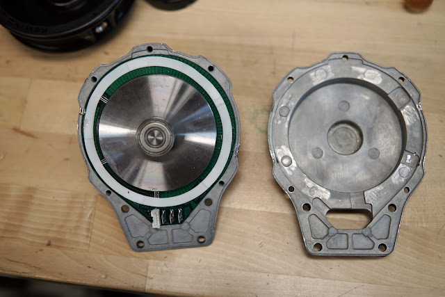
It's a dual-rotor design, with the PCB stator sandwiched between the two halves of the rotor. The rotor is held together by even more retaining compound:

To pull off half of the rotor, I gripped it in a small lathe chuck and used a gear puller to pull it off the shaft:


First a closer look at the stator. The board had at least 4 layers, and probably has 4 oz copper - it's very dense feeling.
Some observations and thoughts:
- Each phase has 4 4-turn coils, and the 3 phases are overlapped. This is a full-pitch winding.
- This winding pattern results in a large area of end-turn, so the actual "active" area of the stator is unfortunately small - less than half the area of the PCB actually produces torque.
- The traces neck down and become thinner within the active area. Presumably this is to reduce eddy current losses from the magnets swinging over the traces.
- The hall sensors are through-hole halls, surface mounted sideways into cutouts in the PCB, so they add almost no additional thickness.
- The empty space around the edges of the board are filled with radial strips of copper. I'm not really sure why. Maybe for thermal reasons? The edge of the board is heatsinked to the aluminum housing through a ring of thermal pad.
Here's the patent for reference.


The two rotors have single-piece magnets magnetized with 4 pole-pairs:


One of the reasons it's all held together with retaining compound is that the bearing bores in the castings aren't even post-machined. The bearing is just glued straight into the rough, tapered hole in the casting:

Back-EMF is pretty sinusoidal. An FFT reveals a little bit of 5th harmonic. Flux linkage is ~.0044, for a torque constant of .0264 N-m/A (peak phase amps). Line-to-line resistance is 125 mOhms. This gives a motor constant of .086 N-m/sqrt(watt).

Over all it's not a particularly high performance motor for it's size or weight. There's a lot of dead space, and a very heavy, high-inertia rotor.
Here's the weed-wacker. I just got the head of the tool- they make a base called the "drive unit", which holds the battery and electronics. Each head has its own motor:

The motor's right at the end, direct driving the spool of wire:

Removed from the stick. Three board-mount faston terminals for phase power, and another connector for hall sensors.

The motor was a huge pain to take apart, as it is pretty much entirely held together with retaining compound. With a hammer and some screwdrivers I was able to pull off the back cover:

The shaft and front bearing were pushed out of the other half of the housing with a gear puller. There's a ring of thermal pad on one side of the board:

It's a dual-rotor design, with the PCB stator sandwiched between the two halves of the rotor. The rotor is held together by even more retaining compound:

To pull off half of the rotor, I gripped it in a small lathe chuck and used a gear puller to pull it off the shaft:


First a closer look at the stator. The board had at least 4 layers, and probably has 4 oz copper - it's very dense feeling.
Some observations and thoughts:
- Each phase has 4 4-turn coils, and the 3 phases are overlapped. This is a full-pitch winding.
- This winding pattern results in a large area of end-turn, so the actual "active" area of the stator is unfortunately small - less than half the area of the PCB actually produces torque.
- The traces neck down and become thinner within the active area. Presumably this is to reduce eddy current losses from the magnets swinging over the traces.
- The hall sensors are through-hole halls, surface mounted sideways into cutouts in the PCB, so they add almost no additional thickness.
- The empty space around the edges of the board are filled with radial strips of copper. I'm not really sure why. Maybe for thermal reasons? The edge of the board is heatsinked to the aluminum housing through a ring of thermal pad.
Here's the patent for reference.


The two rotors have single-piece magnets magnetized with 4 pole-pairs:


One of the reasons it's all held together with retaining compound is that the bearing bores in the castings aren't even post-machined. The bearing is just glued straight into the rough, tapered hole in the casting:

Back-EMF is pretty sinusoidal. An FFT reveals a little bit of 5th harmonic. Flux linkage is ~.0044, for a torque constant of .0264 N-m/A (peak phase amps). Line-to-line resistance is 125 mOhms. This gives a motor constant of .086 N-m/sqrt(watt).

Over all it's not a particularly high performance motor for it's size or weight. There's a lot of dead space, and a very heavy, high-inertia rotor.
Subscribe to:
Posts (Atom)